Capital Budgeting Lecture

Recall the First Principles of Corporate Financial Decisions:

1. Invest in projects that yield a return greater than the minimum acceptable hurdle rate.
    

2. Choose a financing mix that minimizes the hurdle rate and matches the assets being financed.
    

3. If there are not enough investments that earn the hurdle rate, return the cash to stockholders.

In the Capital Budgeting decision arena, any useful decision tool should:

Consider actual cash flows.

Consider timing effectively.

Consider risk.

Be adaptive to different situations.

Be understandable to non-financial types.

Payback Period (PB)

Indicates how long it takes for cash inflows to repay the initial investment in a project.


To Calculate:

If the expected cash flows are all the same, then PB = Initial Cost / CF

Example (Project 1 on the handout): PB = 2000/330 = 6.06 Years


If the cash flows are not all the same, you simply sum the cashflows until the total exceeds the cost of the project. You can use interpolation to narrow the result down to the desired level of accuracy.

Problems with Payback Period:

1. Fails to consider timing effectively (no discounting or cashflows).
    
2. Generally is used with an arbitrary cutoff point.
    
3. Ignores cashflows past the cutoff point.
    
4. Does not directly consider risk .

Discounted Payback Period (DPB)

DPB is very similar to PB except that it uses discounted cash flows instead of non-discounted cashflows. The advantages of DPB over PB are:

1. It provides a better consideration of timing of cashflows.
    
2. It provides a better consideration of risk if the discount rate is chosen correctly.

However, it still may suffer the problems of an arbitrary cutoff point and failure to consider cash flows past the cutoff point.

Average Return on Investment (ROI)

This class of tools includes similar measures with names like Accounting Rate of Return, Book Rate of Return, Return on Book Value, etc. Do not confuse this with the Internal Rate of Return (IRR).

To Calculate:

The example uses a very simple definition: Avg ROI = Avg CF / Cost


Problems with ROI:

1. May not use actual cashflows.
    
2. Ignores (and even masks) timing by using the average cashflow, thus assuming that all cashflows are equal.
    
3. It does not directly consider risk, and even masks variability by using the average.
    
4. It has no standard definition.

Net Present Value (NPV)

NPV is the strongest method for estimating the value of an investment. It effectively incorporates timing and risk, if properly used. Most important, it provides an estimate of the value created or destroyed by engaging in an investment project.

   

NPV > 0 indicates that value will be created.

NPV < 0 indicates that value will be destroyed.
 

NPV Shortcomings:

1. NPV is not easy to understand in its raw state.
    
2. NPV is easily abused.
    
3. NPV is not directly comparable across projects with different costs or lives.
    
4. NPV looks too scientific. Its users sometimes forget that it is only and ESTIMATE that depends on the ASSUMPTIONS on which it is based.

Profitability Index (PI)

Profitability Index allows the comparison of projects with different costs by showing the Net Present Value per dollar of invested capital.

PI is computed one of two ways:

NPV ÷ Project Cost

Present Value of Future Cash Flows ÷ Project Cost

Both provide the same information, but the first method gives a PI greater than zero for positive NPV projects and the second method gives a PI greater than one for positive NPV projects. The decimal portion of both gives the NPV generated per dollar of investment.

While PI helps in the ranking of projects, it cannot be used in isolation. In the presence of a capital constraint, the objective is always to maximize the total NPV of invested capital.

Equivalent Annual Annuity (EAA)

EAA allows the comparison of projects with different expected life spans by providing a measure of the NPV generated per year of a project's life.

The computation of EAA is simply to determine the equal annual payment (annuity) that would have the same present value as the NPV of the project.

For example, consider Project 7 on the handout. It has a 5 year life and an estimated NPV of $165. Its EAA is computed as follows:


PV	-165
FV	0
n	5
i?	10
PMT?	43.53

The EAA lets us think of this project as generating $43.53 of NPV per year rather than thinking of it as generating a one-time NPV of $165. This project can be compared with others with different life spans on this basis.

Internal Rate of Return (IRR)

The IRR represents the average annual expected rate of return on a project.

IRR is defined as the discount rate that makes NPV = 0.

An NPV profile is a graph that relates the NPV of a project to changes in the discount rate. The point at which the NPV profile crosses the horizontal (discount rate) axis gives the IRR of the project.

Advantages of IRR:

1. It is reasonably easy to calculate, especially with a financial calculator or a spreadsheet.
    
2. It is easy to understand, since it represents a percentage rate of return.
    
3. It usually gives the same decision (accept or reject) as NPV.
    

Calculations:

If the project only has one expected inflow and one outflow as in Project 3, the calculation is simply as follows:


PV	-2000
FV	10000
n	15
i?	11.33%
PMT	0

If the project has equal annual cash flows as in Project 5, the calculation is:


PV	-2000
FV	0
n	15
i?	11.12%
PMT	280

If the project has equal annual cash flows with an extra amount at the final period, the calculation is:


PV	-2000
FV	670
n	8
i?	10.87%
PMT	330

If the cashflows do not fit into any of the above patterns, then the use of an NPV profile and some trial and error may be needed.

The decision criteria for IRR is to compare the project's IRR to a hurdle rate, which should be based on the company's risk adjusted cost of capital. 

If IRR > Cost of Capital, then the project will create value if accepted.

If IRR < Cost of Capital, then value will be destroyed if the project is accepted.



IRR Shortcomings:

1. The IRR computation does not necessarily produce a unique solution. That is, there could be more than one IRR for a project, in which case none can be used. An IRR is produced for each change of sign in the cash flow stream.

For example, consider a project that has a $1,000 cost, one expected cash inflow of $1,200 at t=1 and one later inflow of -225 at t=15. The NPV Profile for the project looks like this:

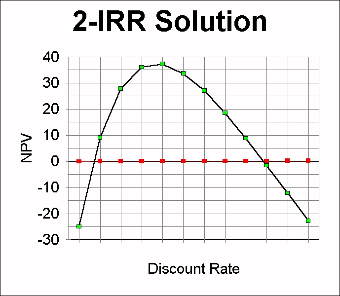
This project has two IRR's -- one at 1.5% and one at 17.5%. In this situation, both are correct and neither are correct. It is best not to use IRR in this case and use just NPV instead.


2. The calculation of IRR assumes that all annual cash flows are reinvested in another project with the same IRR over the remaining life of the investment. This tends to overstate the actual expected return on high IRR projects while understating the expected return on low IRR projects.
    
3. IRR can be easily abused by failing to set the hurdle rate appropriately. The correct hurdle rate is the cost of capital of the company, adjusted for the risk of the project.
    
4. IRR can give an incorrect decision signal (one that differs from the signal given by NPV) if it is used to rank mutually exclusive projects. The example used in class referred to Project 7 and 8. Project 7 has the higher IRR but the lower NPV. The correct ranking is to take the project with the higher NPV per dollar of investment (PI) and per year (EAA).

Modified Internal Rate of Return (MIRR)

MIRR provides a "fix" for some of the shortcomings of IRR while maintaining its desirable characteristics. Its advantages are:


1. It always produces a unique solution.
    
2. It assumes that cash flows are reinvested at the average rate of return (the cost of capital) instead of at the IRR. This produces a more conservative estimate of the the average annual expected return on the project.
    
3. It produces a more dependable (but not perfect) ranking of mutually exclusive projects.
    

Calculation of MIRR:

1. Compute the total future value of all cash flows (except the one at time zero) at the last year of the project's life. Use the appropriate discount rate (the risk-adjusted cost of capital) to compute this future value.
    
2. Compute the annually compounded rate of interest that relates the total future value to the project's initial cost. This is the MIRR for the project.

For example, consider Project 2:


Time	CF	FV
1	1666	2015.86
2	334	367.40
3	165	165
	Total FV	2548.26




PV	-2000
FV	2548.26
n	3
PMT	0
i?	8.41

---

What Firms Actually Use

Damodaran Text Table10.11 Page 312

Technique	Primary		Secondary
	Number	Percent	Number	Percent
IRR	288	49	70	15
ARR	47	8	89	19
NPV	123	21	113	24
PB	112	19	164	35
PI	17	3	33	7
Source: Kim, Crick, and Kim (1986)

 

Payne, Heath, and Gale; Journal of Financial Practice and Education - Spring/Summer 1999

IMPORTANCE OF TECHNIQUES
ACROSS ALL US RESPONDENTS

Technique	Rank	Relative Rank
IRR	1	1.73
NPV	2	2.00
PB	3	2.59
DPP	4	3.34
ARR	5	3.53
MIRR	6	3.97

 

IMPORTANCE OF TECHNIQUES
BY SIZE OF RESPONDENT

Technique	Quartile 1 (Smallest)	Quartile 2	Quartile 3	Quartile 4 (Largest)
PB	1	2	3	3
DPP	3	3	4	4
ARR	4	3	5	5
IRR	2	1	2	2
MIRR	4	4	6	6
NPV	1	2	1	1

 

---

Capital Budgeting Framework

Uses:

Incremental Analysis
After tax cash flows
Operating cash flows only


Test for inclusion of cash flows:

Does a change in the accept/reject decision change the cash flow in question?



---

Net Initial Outlay:

-	Price of new asset
-	One-time costs
+	Sale of existing asset(s)
+-	Tax effect on sale
+-	Change in NWC
-	Opportunity costs
	Net initial outlay

Note: The sign on "CHANGE" is determined by (New - Old)

Caution: Do not include sunk costs!



---

Periodic (recurring) Cash Flows:

Note: Watch for opportunity costs, sales erosion, and allocated overhead.

Terminal Cash Flows: